Detecting Behavior from Timeseries Data

If you want to score behavior in a video, you can either scroll through the entire video by hand (slow, monotonous), or you can pre-detect movements and then validate them (80–90% faster).

CodeNeuro provides tools to do the latter.

We first transform the video into a timeseries, where each timepoint represents a frame of the video. Then we apply an algorithm to detect the onset of events.

This post dives into the algorithm used to detect events from timeseries data.

The final product

Baseline Estimation

Before we can detect events, we need a threshold. Values above this threshold will be considered movement.

But this has to work across a variety of timeseries data. Not an easy task.

Naive baselines

A naive approach would be to use the mean or median of the data. And depending on the timeseries, that could work.

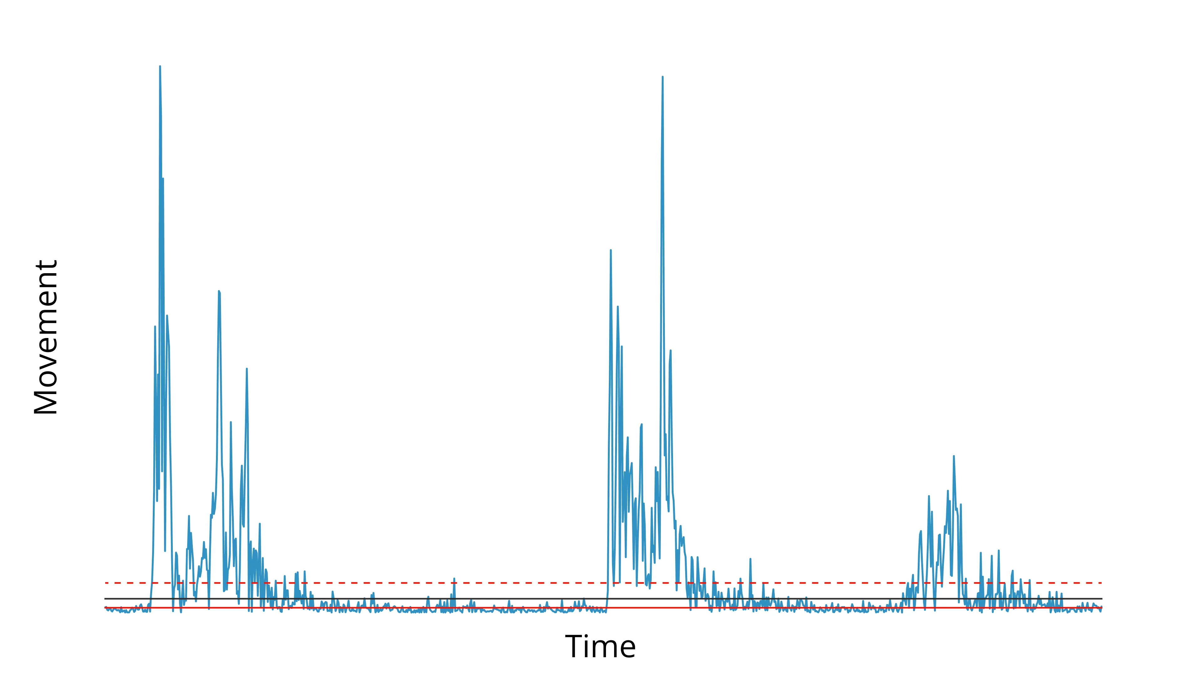
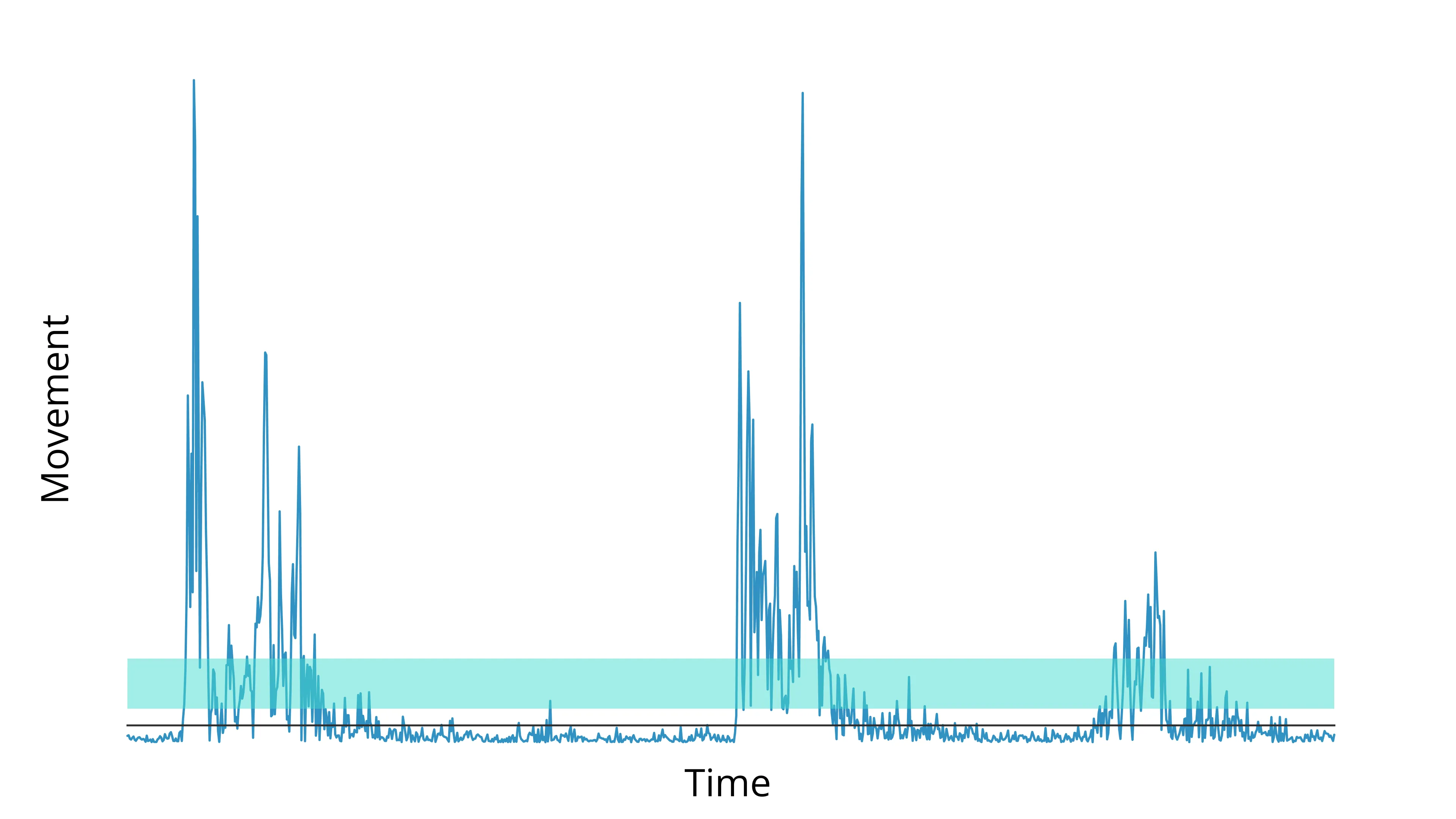
Let’s look at the “noise band” of the timeseries below.

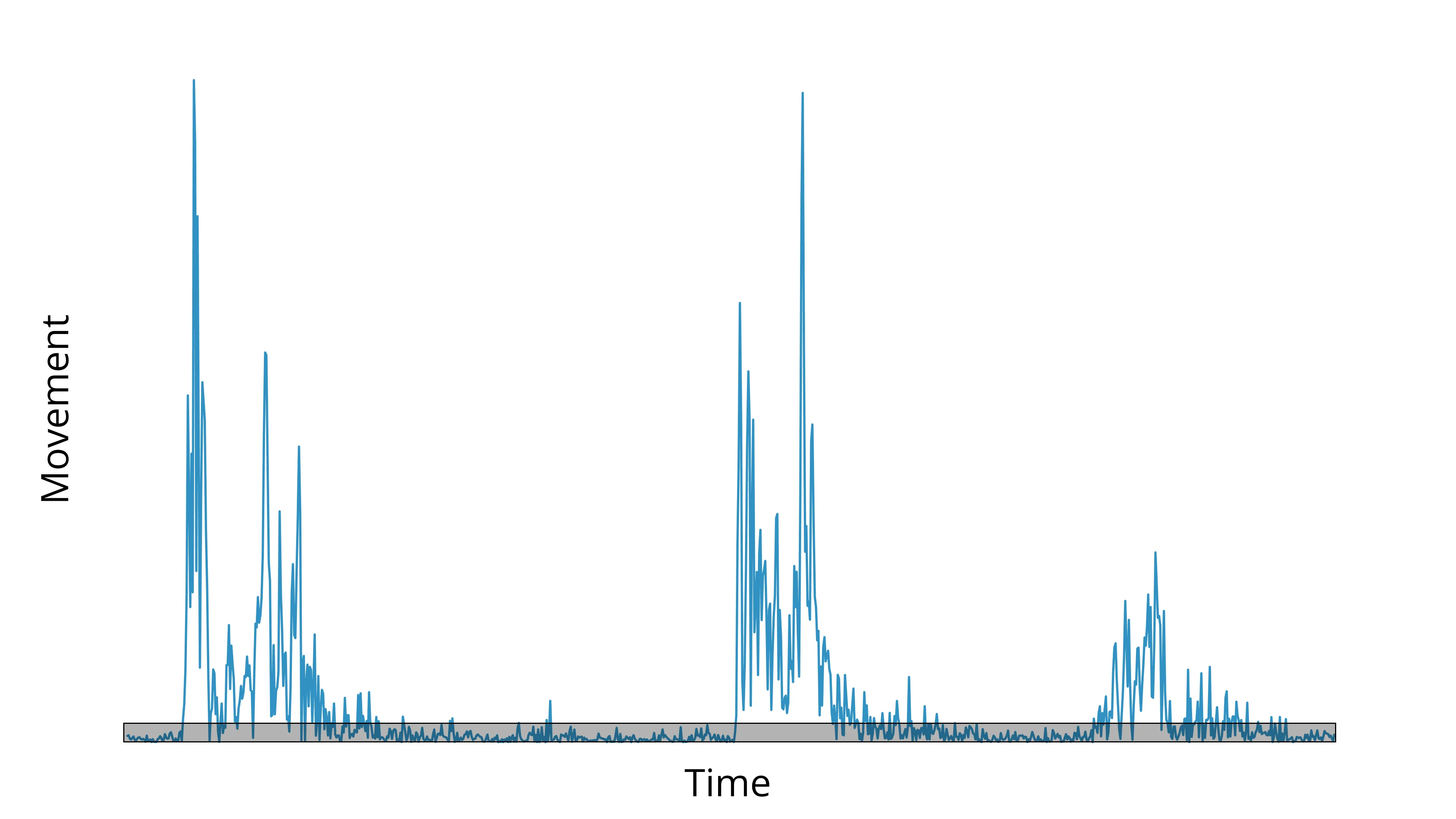
Noise band, highlighted in gray

We want to estimate the top of that noise band, then set a threshold 2–5x higher than that.

Notice that neither the median (solid red line) nor mean (dashed red line) provides a great estimate of the noise band.

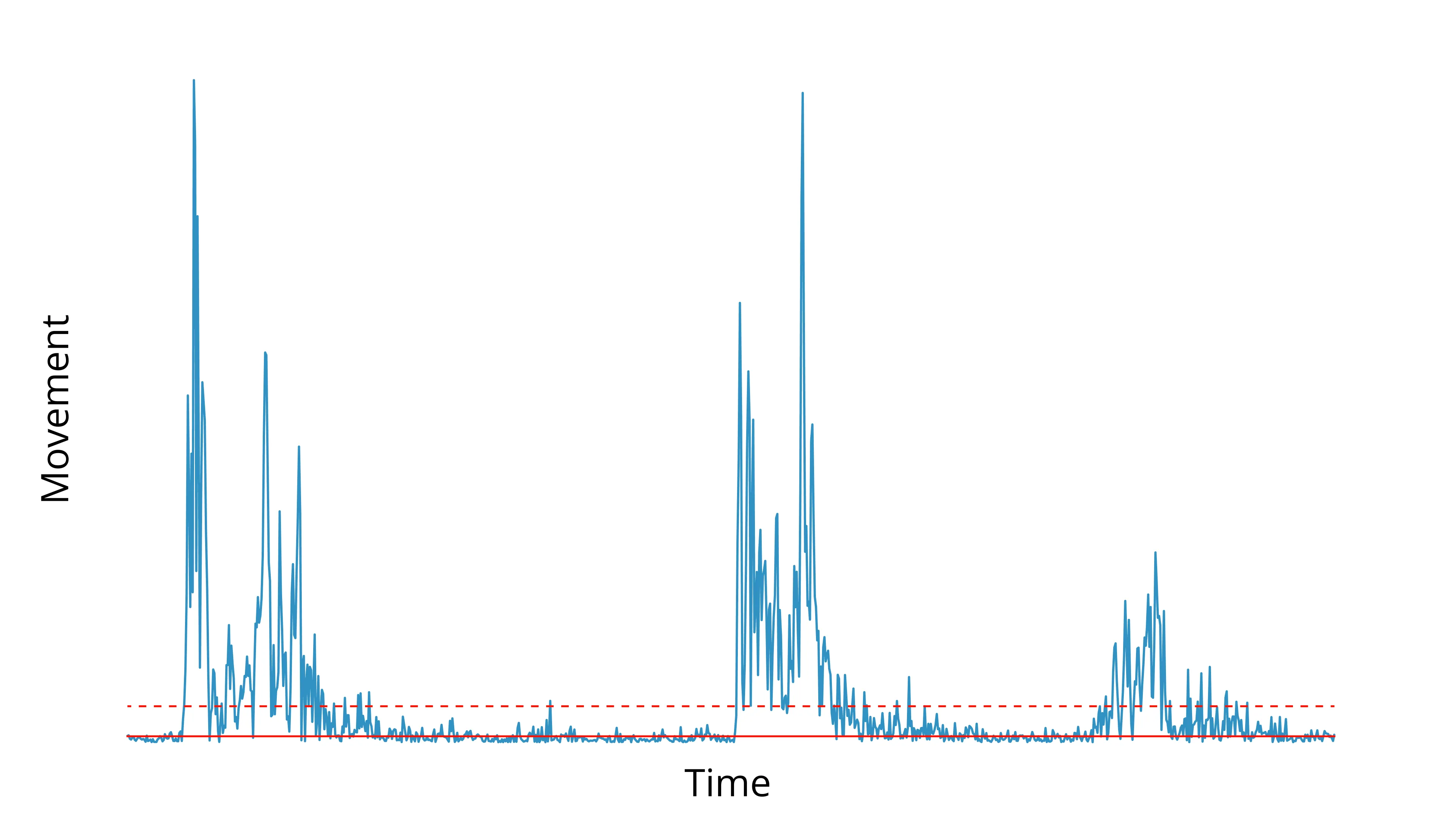
We could compensate for that by using the median and picking a high multiplier for the threshold, or vice versa for the mean—but that rarely pans out well across videos.

Instead you end up really missing the mark on videos that have higher or lower than normal noise.

Instead, we take a custom approach to estimating the baseline. It works better.

Custom baseline

First, we split the timeseries into 100 ms bins.

def estimate_baseline(timeseries, fps):
    bin_size = round(fps * 0.1)  # 100 ms
    bounds = len(timeseries) // bin_size * bin_size
    bins = timeseries[:bounds].reshape(-1, bin_size)
    ...

Then we find the top of each bin. We will take advantage of the fact that the vast majority of bins contain only the noise band.

(To avoid extreme positive outliers, we take the 95th percentile rather than the maximum.)

def estimate_baseline(timeseries, fps):
   ...
    heights = np.nanpercentile(bins, 95, axis=1)
    heights = heights[~np.isnan(heights)]
   ...

Next, we compute a kernel-density estimate (KDE), which models the distribution of all bins.

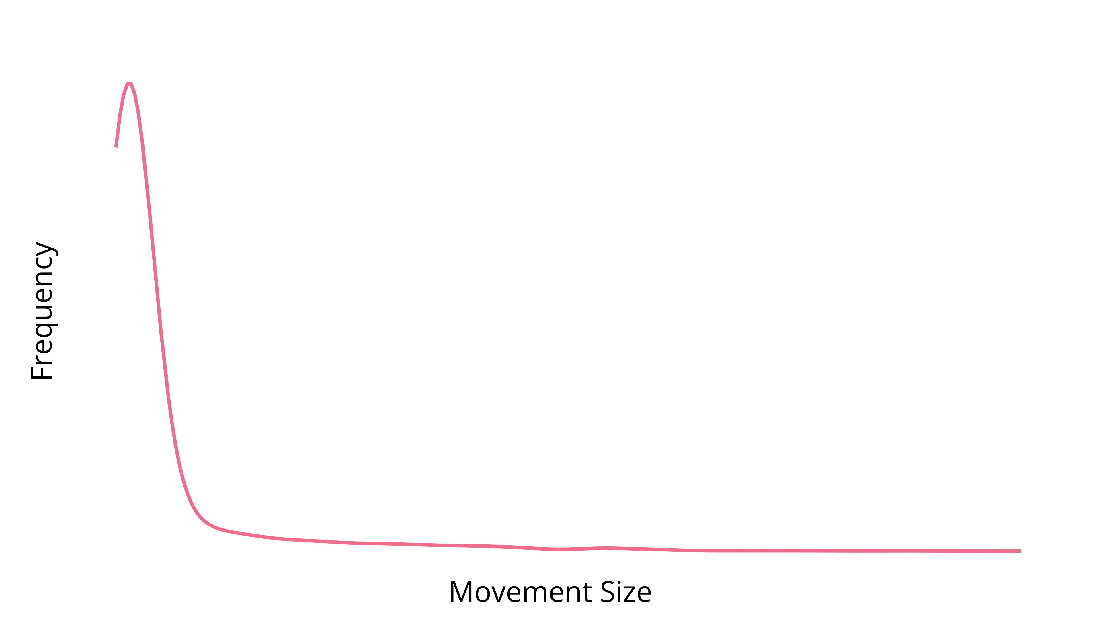
That spike is the modal value of the 95th percentile of the bins, a.k.a, the modal noise-floor height.

This is our baseline estimate.

def estimate_baseline(timeseries, fps):
    ...
    try:
        kde = gaussian_kde(heights)
        x = np.linspace(heights.min(), heights.max(), 1000)
        baseline = x[np.argmax(kde(x))]

        if baseline > 0:
            return baseline
    except Exception:
        pass
    ...

You’ll notice there are a couple guards in that code—if the baseline is 0 or an exception occurred, we proceed with a fallback. The KDE is a pretty resilient calculation, but some datasets can cause it to falter.

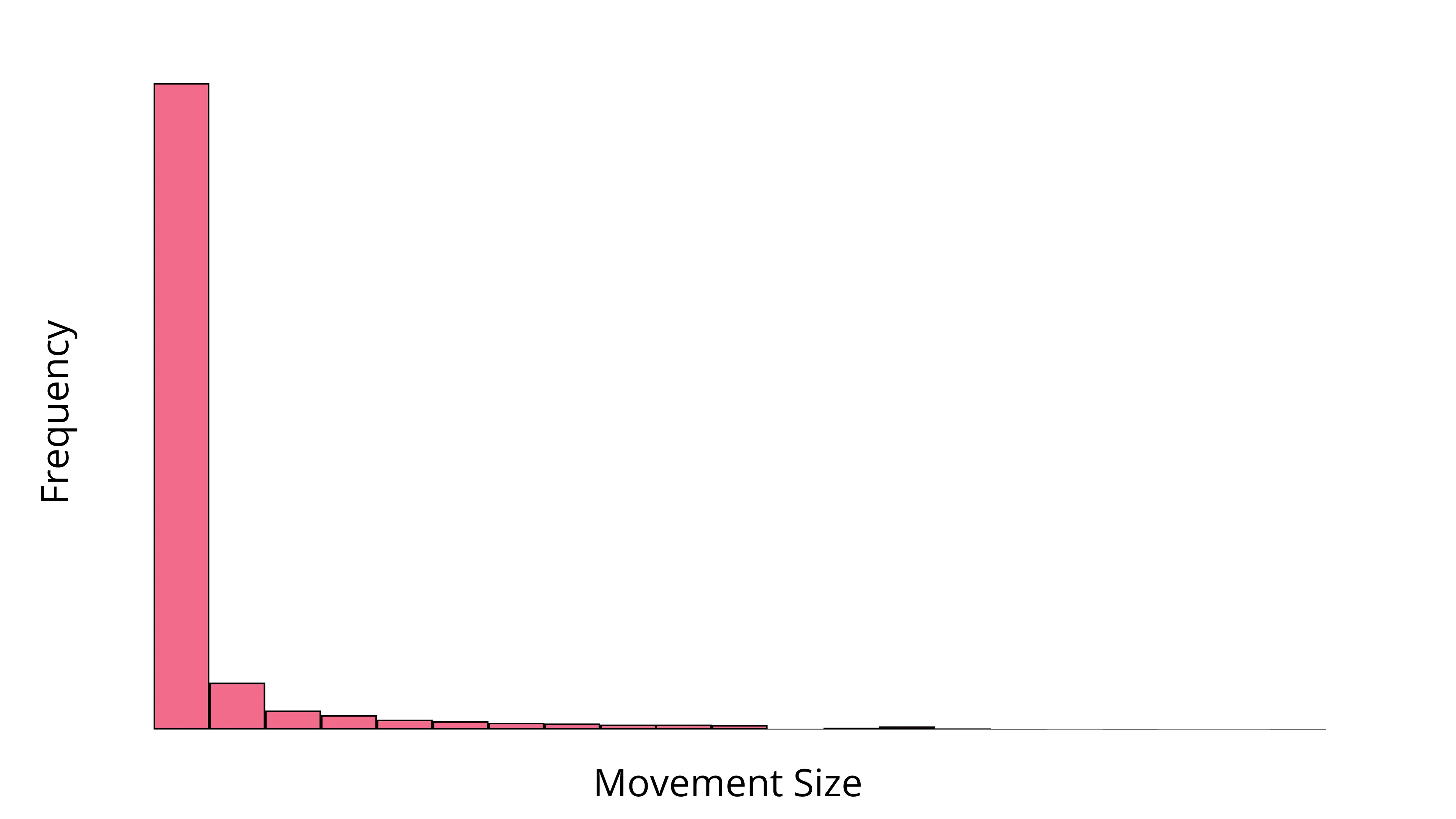
The fallback is a simple histogram which approximates the same thing as the KDE.

def estimate_baseline(timeseries, fps):
    ...
    hist, edges = np.histogram(heights, 100)
    highest_bin = np.argmax(hist)
    baseline = np.mean(edges[highest_bin : highest_bin + 2])
    return baseline

Here is the full code for the baseline estimation:

def estimate_baseline(timeseries, fps):
    bin_size = round(fps * 0.1)  # 100 ms
    bounds = len(timeseries) // bin_size * bin_size
    bins = timeseries[:bounds].reshape(-1, bin_size)

    heights = np.nanpercentile(bins, 95, axis=1)
    heights = heights[~np.isnan(heights)]
    try:
        kde = gaussian_kde(heights)
        x = np.linspace(heights.min(), heights.max(), 1000)
        baseline = x[np.argmax(kde(x))]

        if baseline > 0:
            return baseline
    except Exception:
        pass

    # Histogram fallback
    hist, edges = np.histogram(heights, 100)
    highest_bin = np.argmax(hist)
    baseline = np.mean(edges[highest_bin : highest_bin + 2])
    return baseline

Now that we have a baseline estimate, we set a threshold (2–5x works well; CodeNeuro uses 3x by default) to detect events.

Peak detection

We use SciPy’s find_peaks method to detect local maxima in the timeseries, then the peak_prominences method to measure the height of the peak compared to the neighboring points (to assess movement relative to current displacement, not relative to zero).

Notice that only the left prominences are calculated—we only care about what happens before this displacement, not after.

Next, we remove any prominences below the threshold and apply an onset time kluge (little fix)—because we are not interested in peak displacement, but rather movement onset, we subtract a single frame.

def detect_left_tail_peak_prominences(timeseries, threshold=3):
    peaks, _ = find_peaks(timeseries)
    if peaks.size == 0:
        return []

    _, left, _ = peak_prominences(timeseries, peaks)
    valid = timeseries[peaks] - timeseries[left] > threshold
    return [p - 1 for p in peaks[valid]]  # shift onset

Rate Limiting

Below is the output of our detect_left_tail_peak_prominences method:

We have one last problem to solve—nearly everything over the threshold was detected as movement!

Depending on the frame rate of your camera, you may notice a significant amount of variation in your timeseries within a single movement. That’s a problem, because we are only concerned with the onset of the behavior, not every tiny change in speed or displacement.

To fix this, we borrow a method from networking called rate limiting. When you try to make too many requests to a website, you may get rate limited, meaning you are blocked until a certain time of inactivity passes.

Here, we apply the same logic:

def apply_rate_limit(events, fps):
    window_size = np.floor(fps * 0.25)  # 250 ms
    s_events = np.sort(events)

    to_limit = np.where(np.diff(s_events) < window_size)[0] + 1
    rate_limited = np.delete(s_events, to_limit)
    return np.unique(rate_limited).tolist()

When a flurry of detected movements begin, we keep the first movement.

Then, we discard any movement that occurs within 250ms of the previous movement (not just the first!).

E.g., if movement are detected at +0 ms, +100 ms, and +300 ms, we will throw out all but +0 ms.

Yes, +300 ms - +0 ms > 250 ms. However, there needs to be a “quiet period” of 250 ms before a movement occurs (and +300 ms - +100 ms = 200).

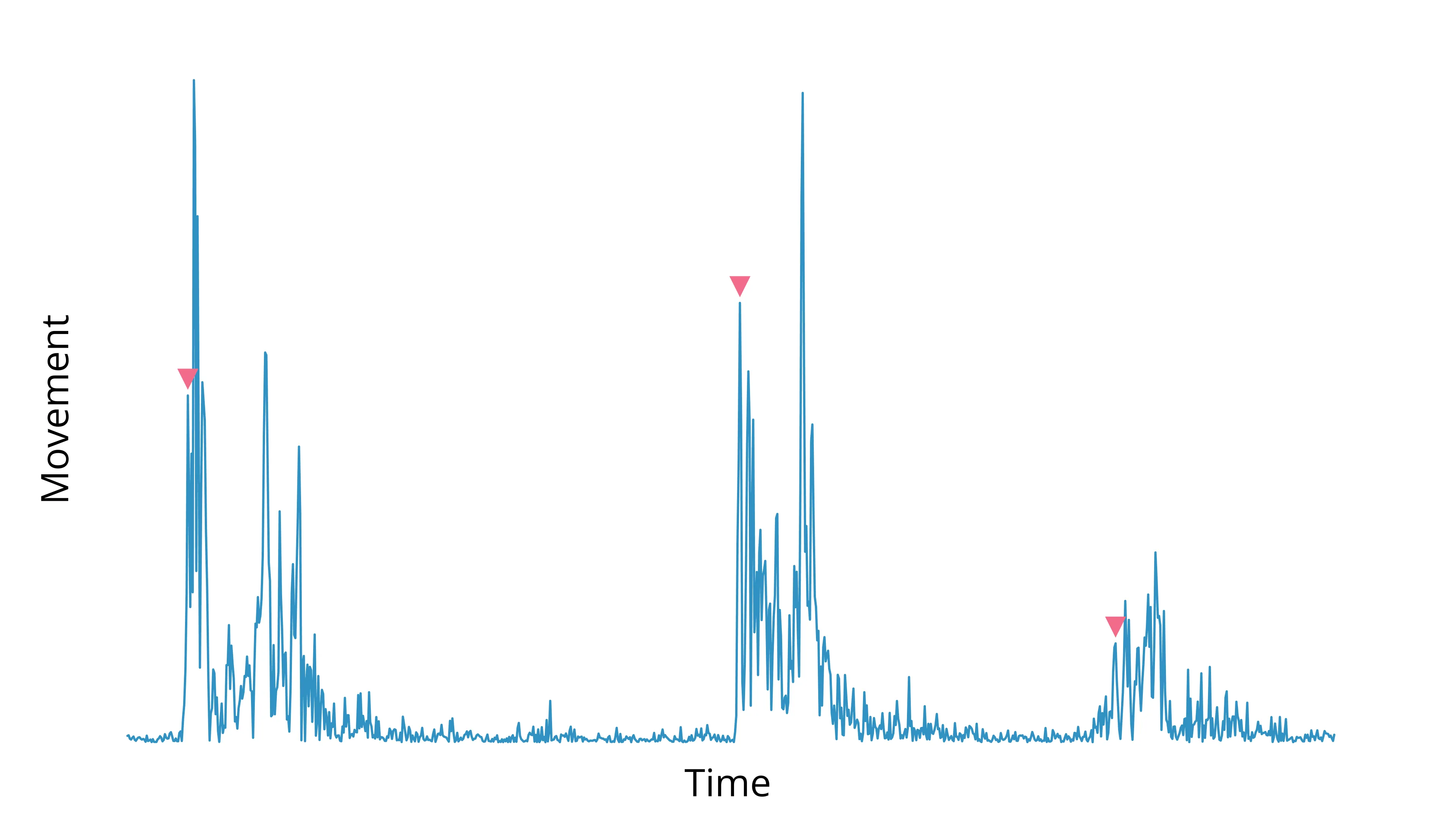
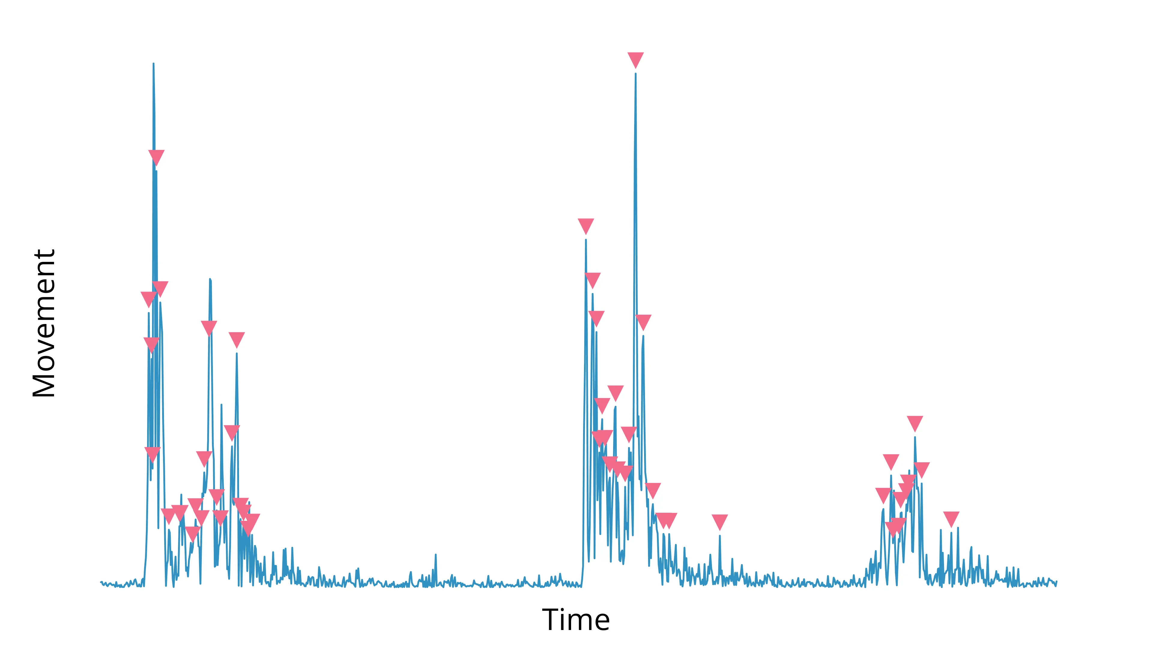
When we apply this step, we finally get a clean detection of behavior onset times:

Conclusion

This is how we detect the onset of behavior based on our movement detection algorithms or a timeseries that is imported to CodeNeuro.

Of course, this is all unsupervised. For clean behavioral data, you must verify the timestamps yourself. We recommend our Quick Score tool, which allows you to accept, adjust, or discard each event, well, quickly.

The algorithmic-detection → manual validation approach can result in an 80–90% speed-up compared with a fully manual detection approach and keep your behavioral data just as trustworthy.